Optimizing Streaming JOINs: Leveraging Asymmetry for Better Performance

When describing the core SQL (Or relational algebra) operators, the humble join shows up pretty fast. In fact, you would be hard pressed to find an app built on top of an SQL database which doesn’t use a join in one of its queries. For good reason! Joining two sets of data based on some predicate is the basis for creating any sort of relation between logical entities, whether it is one-to-one, one-to-many, etc.

At Epsio, we’re building a fast, streaming SQL engine which computes the result of arbitrary SQL queries in real time, based on changes. So, it’s no surprise that we’re very motivated to have an optimized implementation of join. In this post we’ll describe a key idea that allowed us to optimize our streaming join in common cases.

But before we dive into optimizations, let’s first describe how the Symmetric hash join algorithm, which is commonly used in stream processing, works. We will only discuss inner join in this post for simplicity, even though there is a lot to talk about other join types.

Background: Symmetric Hash Join

Let’s say that we are running a bookstore, and there are 2 tables in our sales database: customer and store_sales. Each row in the customer table has a unique id primary key along with a name column. To connect customers with sales, each store_sales row has a buyer_id column pointing to the relevant customer, and a book_name specifying the book name. We can visualize this relation like so:

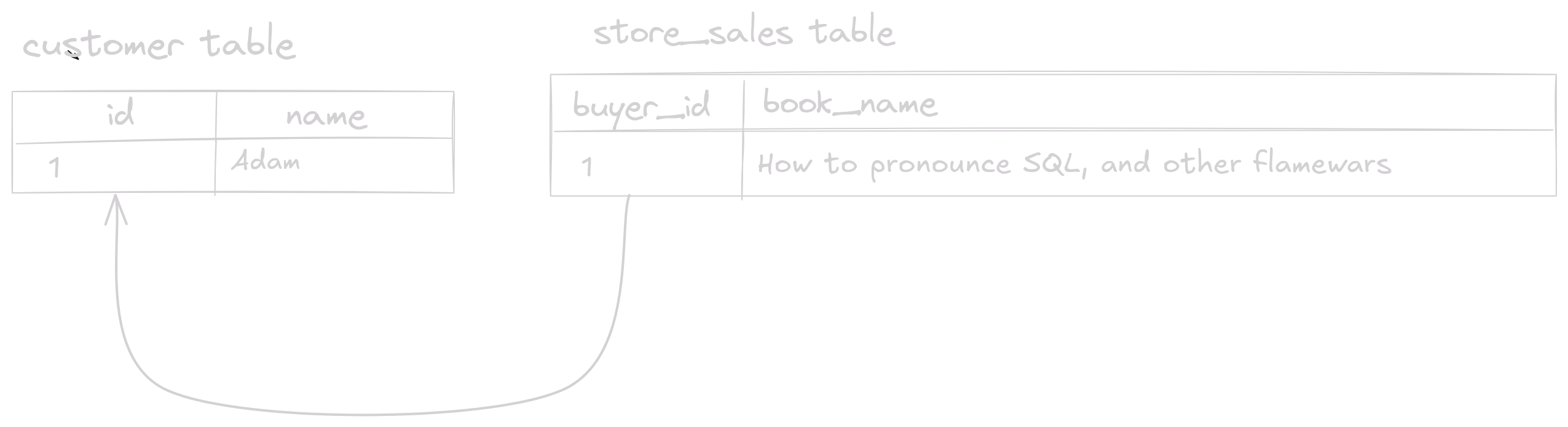
If we want to retrieve all the customers with the book names they bought, our query would look like this:

SELECT customer.name, store_sales.book_name FROM customer
JOIN ON customer.id = store_sales.buyer_id;

The result in this example would be a single row: ("Adam", "How to pronounce SQL, and other flamewars").
How can we implement this join?

If we have all the data ahead of time, A naive solution could be to first build a hashtable for store_sales keyed by buyer_id . We would then iterate over each row in customer, reading the matching sale. In Python:

# Build the store_sales hashtable
for sale in store_sales:
    store_sales_hashtable[sale.buyer_id] = sale.book_name
# Probe the store_sales hashtable using customer
for c in customer:
    if c.id in store_sales_hashtable:
        sale = store_sales_hashtable[c.id]
        output_result((c.name, sale.book_name))
   

This is the classic hash join algorithm.

In a streaming context however, things get more complicated. We don’t have all the data ahead of time, but instead receive live changes. This means that e.g whenever a new sale is added, the streaming engine receives a change message containing the new row just added to store_sales. It then needs to understand how this changes the query result, and issue an update to the previous result accordingly. In the case of our join example, this looks like this:

We had received a new sale, with buyer_id=1. So we need to check if we have a customer with id=1, and if so retrieve their name to return the correct result.

This is exactly where our classic hash join fails. We build a hashtable for store_sales, but we have no state for customer. In the classic algorithm, we can probe the hashtable using the full data of customer table. Here we don’t have the entire table available, since we are working based on changes and don’t have all the data up front. Thus we won’t be able to find the matching customer for our sale.

If we flip the roles and only build a hashtable for customer instead,  we encounter a similar problem. Assume that instead of adding a sale we receive the following change: The name of “Adam” had changed to “Adam, for real” (as so happens). Our new result would then look like this:

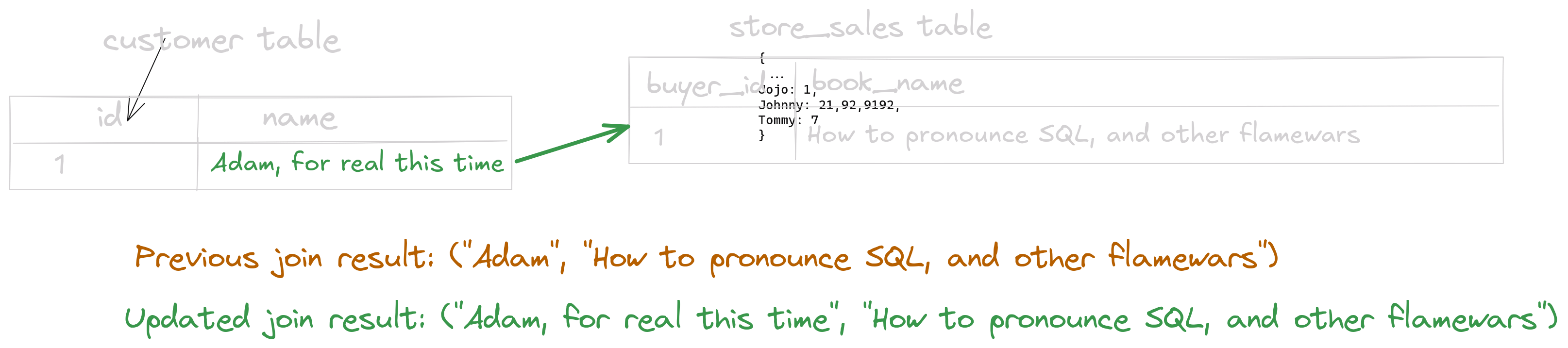
But if we only store a hashtable for customer, we will not be able to find the matching store_sales rows when the change is received! Luckily, there is a simple change that solves our problem.

Well, like many other problems in  computer science, this one is also resolved by adding another hashtable. In particular, we maintain two hashtables: one for customer keyed by id, and another for store_sales keyed by buyer_id.

Now whenever a new customer is added, we lookup the store_sales hashtable by the customer id to return the matching sales. We then write the customer to the customers hashtable, to ensure that it is visible for future lookups for when another sale is added.

The other direction is similar: when a new sale is added, we lookup the matching customer in the customer hashtable to see who bought the item. We then write the new sale to the store_sales hashtable.

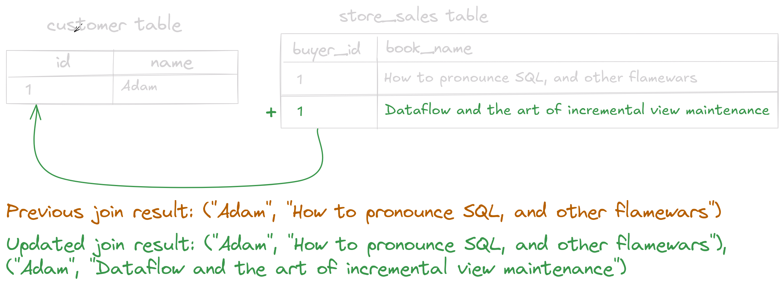
So  when Adam buys a new book, we lookup the customer hashtable with buyer_id=1 and write the new sale:

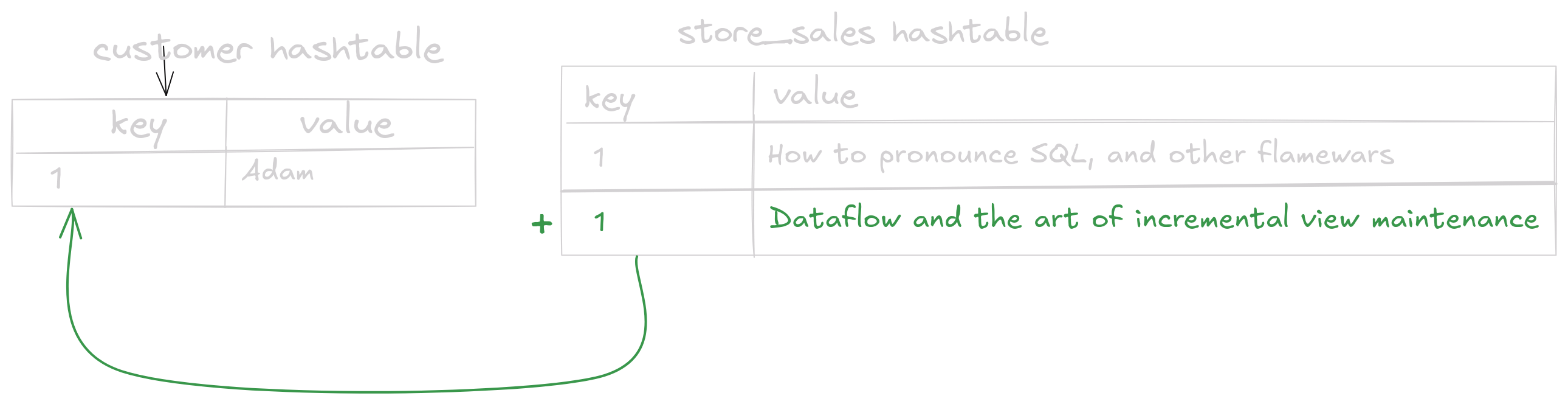
We will then return the new result row ("Adam", "Dataflow and the art of incremental view maintenance"). This is the essence of the Symmetric Hash Join (or SHJ for short) algorithm: on a change to one side of the join, write the change to the hashtable of this side, and then read the matching rows from the hashtable of the other side to get the matching row. Pretty simple, right?

The Population Problem

This algorithm is the core join algorithm used in Epsio. There is one key detail we have glossed over though: Most of the time, the hashtables for the 2 join sides don’t fit in memory. We need to have persistency to be able to do the join with reasonable data sizes.

This is a perfect candidate for using a Key value store: Our key is the join key, and the value is the row. In particular, we use the rock-solid RocksDB to save the join states, with each state in a separate RocksDB database. As RocksDB plays a big role in optimizing our join implementation, we will describe it in more detail below.

Another important detail, and what brought us to look closer into join optimization,  is the population phase. Epsio, like other streaming engines, has an initial data load phase. Before we can respond to live changes to data and update the query result, we must first compute the result for the existing data in the user’s database. We also need to populate our inner states, like the join hashtables, so that we could stream changes to compute updated results. This phase can  be a computationally intensive task, since the initial amount of data can get quite large.

We have noticed that with many joins in the query, our population time isn’t meeting our expectations. When thinking about it, this isn’t surprising: During population, we can receive hundreds of thousands of rows as input into one join at a time, with different keys. Following the SHJ algorithm as described above, we will be performing these 2 steps a lot:

1. Lookup a key in a RocksDB database. This will be Disk I/O once the join database is large enough.
2. Write a the join key and its corresponding rows to another RocksDB database. The Disk I/O likely won’t be done immediately, as RocksDB flushes data to disk in a separate thread as detailed below.

These 2 steps make the symmetric hash join both a write intensive and a read intensive operation. No wonder that it’s a big part of our population time! Given the importance of join, we started profiling to see how we can improve its performance.

Let’s rock!

To get an accurate picture for where we can improve, we benchmarked the population of a TPC-DS query with many joins, query4. Here’s a shorter version of it with the key details:

 select 
       c_customer_id, 
       d_year,
       sum(ss_ext_list_price - ...) year_total,
       's' sale_type,
       ...
from customer
   join store_sales on c_customer_sk = ss_customer_sk
   join date_dim on ss_sold_date_sk = d_date_sk
group by c_customer_id ,d_year, ...
union all

select 
      c_customer_id,
      d_year,
      sum(cs_ext_list_price - ...) year_total,
      'c' sale_type,
      ...
from customer
   join catalog_sales on c_customer_sk = cs_bill_customer_sk
   join date_dim on cs_sold_date_sk = d_date_sk
group by c_customer_id, d_year, ...
union all

select c_customer_id,
       d_year,
       sum(ws_ext_list_price - ...) year_total,
       'w' sale_type,
       ...
from customer
   join web_sales on c_customer_sk = ws_bill_customer_sk
   join date_dim on ws_sold_date_sk = d_date_sk
group by c_customer_id, d_year, ...

(There is also another inner self-join later in the query, but we can ignore it for the purpose of our analysis here).

The goal of this query is to compute the yearly total purchases per customer, across different sales channels: store_sales, catalog_sales and web_sales. For this purpose, there is a join between customer and each of the sales table, along with a join of the date_dim dimension table with every sales table. This gives a total of 6 joins in the core of our query — perfect for analysis!

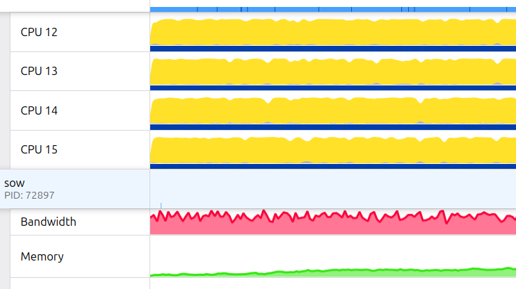
When looking at profiles for this query, we quickly noticed that RocksDB is a bottleneck. For example, writes to the databases of the different join sides  would take a very long time. We started tackling this by looking into the usual suspect: Tuning RocksDB configuration. This worked well and resolved our long running writes, but we were still left with much room for improvement.

Studying the flamegraph more carefully, we found it. The ancient curse. The one that will strike fear into the heart of even the most experienced RocksDB users. The word that was hanging in the air since the start of this post like Chekhov’s merge-sort, the one they have all guessed by now but hoped it wouldn’t show up. The creature lurking in the background threads, in all its glory. Compaction!

What’s compaction, or: Where did my CPU cycles go?

(If the sentence “We need to compact L0 to reduce our read amplification” makes sense to you, feel free to skip this part)

To understand what’s happening, we first need to take a detour and understand how RocksDB stores data. This is a topic for its own blog post, with many resources already covering it. We will give a short summary of the read and write flows to see why we need compaction.

Whenever a new (Key, Value) pair of bytes is inserted to a RocksDB database, it is first written to an in memory data structure called a memtable. This data structure is usually a Skiplist, but all that matters is that it is a sorted list of (K, V) pairs. Once a memtable exceeds its configured capacity, 64MB by default, it is marked as immutable. A new active memtable is created in its place, while the immutable memtable is “sealed” and inserted into a queue of memtables waiting to be flushed to disk. The memtables are flushed in the background to not stall writes.

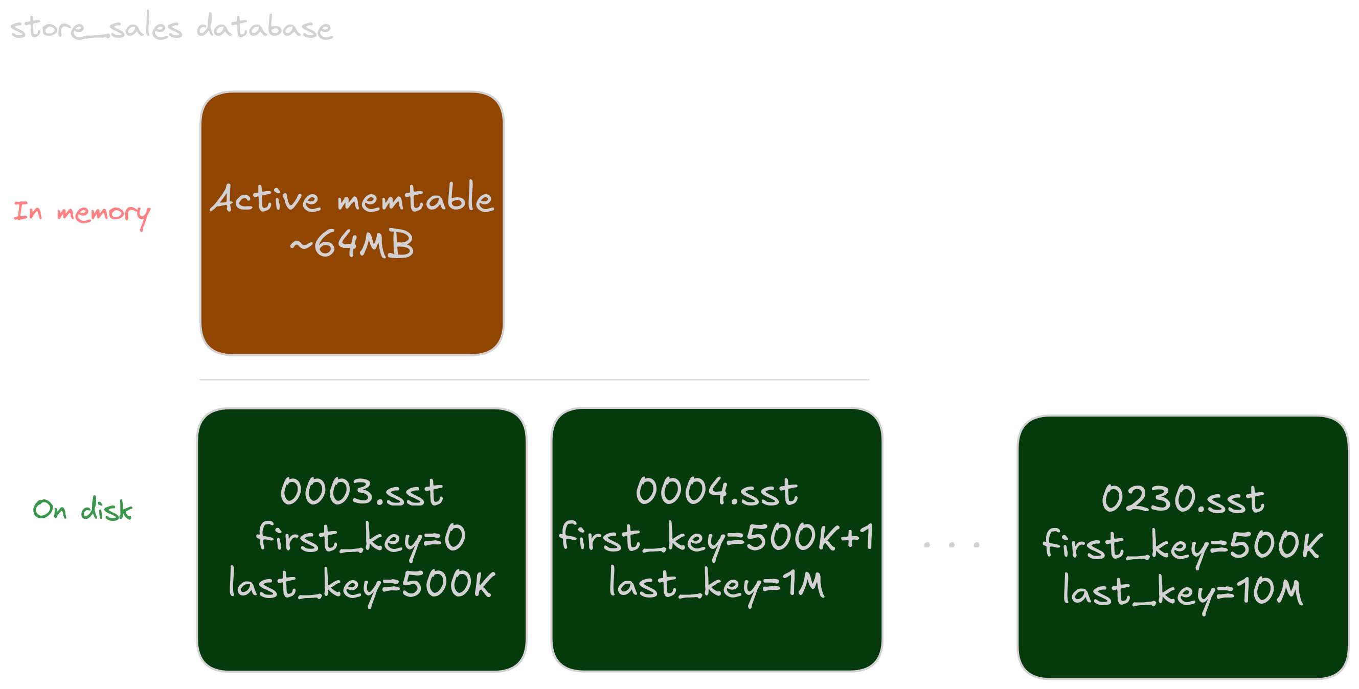
A memtable is flushed to disk as an SST file. The specific format doesn’t matter here much, but the main point is that the each SST is sorted, and thus has a first and last key in some order. For example, at some point in time the store_sales database can look like this:

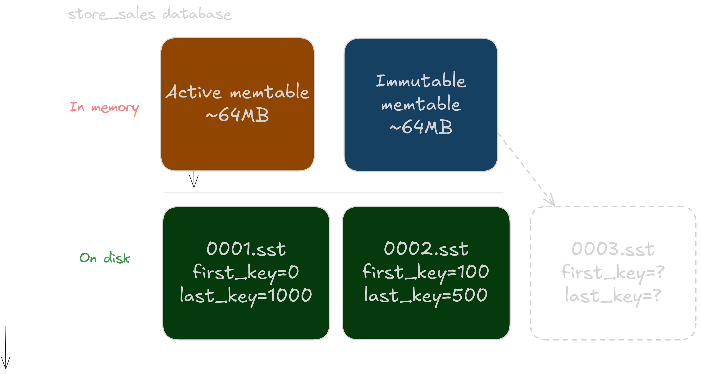
Notice that while both SST files are sorted, their key ranges are overlapping. Indeed, so far we haven’t described some intentional merging of sorted data. If our keys aren’t arriving in a sorted order, which happens most of the time, we will naturally have multiple sorted but overlapping files on disk.

So what does this mean for our read flow? If we want to find a key K, we will have to:

1. Do a binary search on the active memtable
2. If not found, do a binary search on all immutable memtables
3. If not found, perform a binary search on every SST file, loading blocks from disk for search

Step 3 is where we will suffer from key overlap the most. We have to check every SST file for our key, where the amount of SST files can be in the thousands. Lots of I/O, lots of waiting for our KV pair. How can we speed this up?

This is where the Compaction background process comes into play, which occurs in any LSM-tree based database and RocksDB in particular. Its main purpose is to merge multiple overlapping SSTs into non overlapping files (and deleting entries, but this is out of scope for our insert only population flow).

There are several compaction algorithms, with complicated conditions for what to compact, when and how. This is an entire (interesting!) field of research which we will not get into here. Suffice to say that the compaction process will write new SST files instead of the existing ones, performing a merge sort so that we have a sorted “run” of data:

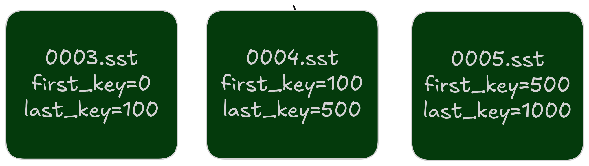
Now when we’ll lookup a key, we will only have to search one SST. Nice!

But there’s a catch. Compaction is an intensive process by itself. We read many SST files, perform a merge sort on a large amount of keys, and write possibly many SST files back. In RocksDB, compaction happens in background threads, causing the many BGThread samples we saw above.

There are many strategies to reduce compaction overhead in RocksDB and in general, but you can’t avoid its overhead entirely. Or can you?

Disabling compaction for bulk load?

Because of high compaction overhead, it is common advice to disable compaction in bulk load cases like our join during population, and do one large compaction at the end of population. Sadly, this didn’t work for our use case: empirically we didn’t see much of an improvement from it. We also can’t avoid compacting for too long; As noted above, the join algorithm is also read intensive: we write to one join side database and immediately read from the other. If we don’t compact, our read performance will suffer.

At this point we started looking a bit more into the data for our specific benchmark, TPC-DS query4, in the SF100(=A raw size of ~100GB) version of the dataset. We then noticed something interesting..

The asymmetry of joined tables

As you may remember, as part of the query we had a join of customer with 3 sales tables: store_sales, catalog_sales and web_sales. We checked the row count for each of these tables, and found out these numbers:

• customer: 2M rows
• store_sales: ~288M rows
• catalog_sales: ~144M rows
• web_sales: ~72M rows

The customer table is much smaller than the tables it is joined with! Anywhere from 36x to a 144x size difference. This isn’t a TPC-DS specific thing of course. One of the use cases of join is to model one-to-many relations, in some cases one-to-much much more.

This is great news for us! Even though the symmetric hash join algorithm itself is, well, symmetric, our data is not. This means that one side of the join will be write intensive, and the other side will be read intensive. So how can we use this asymmetry to our benefit?

Using the asymmetry to minimize compaction overhead

This unlocks many possible optimizations, the one relevant for our compaction problem is: When one side of the join has finished populating, stop compacting the other side.

Why does this work? Let’s look at the customer and store_sales join again, with sizes of 2M and 288M rows, respectively. We have much less customers than sales, so at some point all of our customer rows had arrived, and compaction had finished for the customer database:

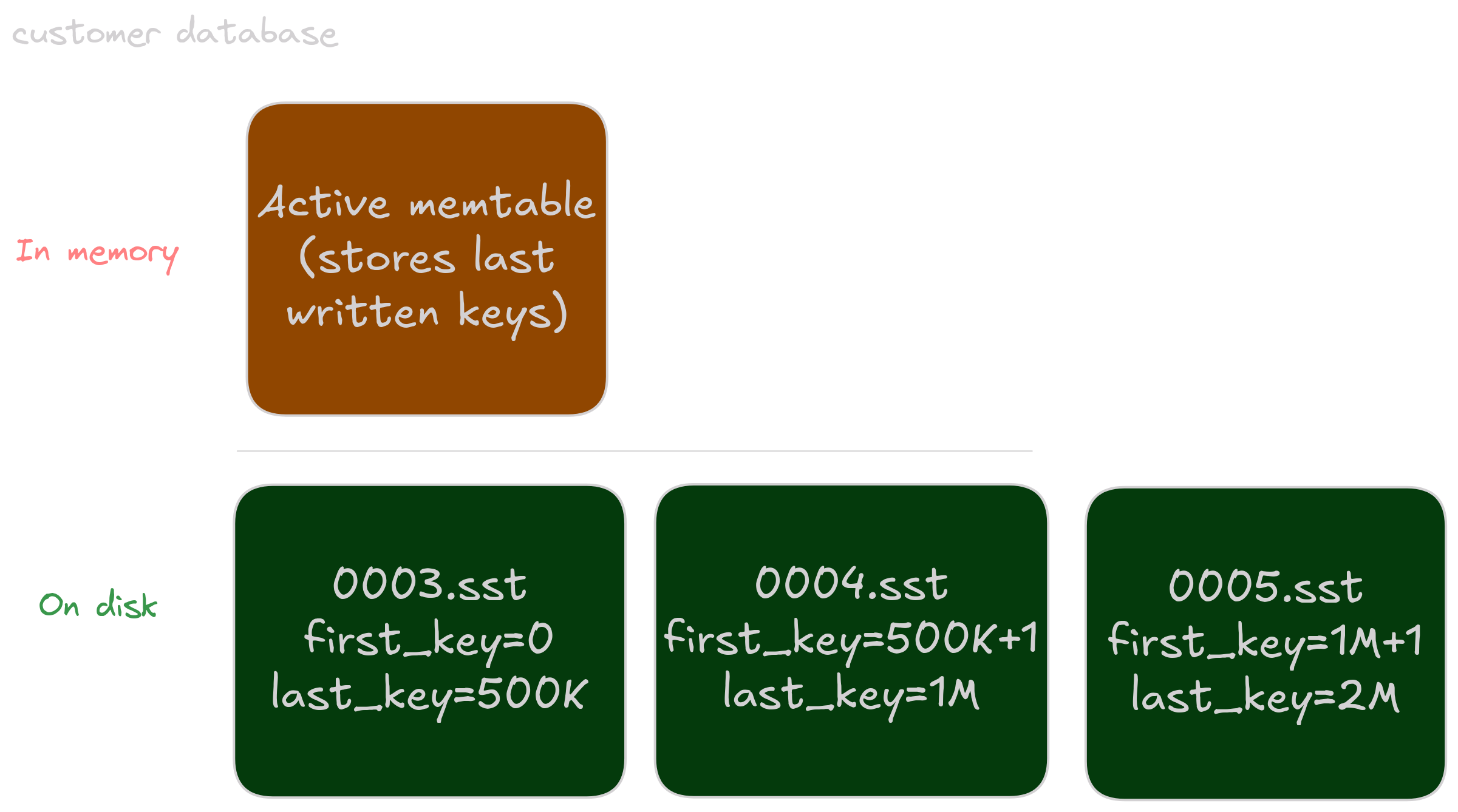
At the same time, new store_sales batches of rows keep arriving, creating more SSTs. Once the last customer had been written to the database, we stopped compacting store_sales, causing an overlap with the newer files written:

However, this doesn’t matter. From this point we are only writing to store_sales, and reading from the already compacted customer. Thus we get to both write and read fast without paying for unnecessary compaction.

We went to  implement this optimization, and  noticed a roughly 1.5x improvements in population times of join heavy queries! That’s awesome, but can we do better?

Can we exploit the asymmetry further?

The insight regarding join sizes enables other interesting optimizations that are possible. For example, in RocksDB the memtable type can be specified. One memtable type that we mentioned earlier is SkipList, which allows concurrent writes but has O(log n) lookup cost. Another one is HashSkipList, Which as the name suggests is a hashtable where the bucket is a skiplist. The HashSkipList type doesn’t support concurrent writes, but has an (amortized) O(1) lookup speed.

Perhaps we could use the fast write yet slightly slower read SkipList for the larger join side, and the slower write but faster read HashSkipList for the smaller join side?

Honestly, we don’t know yet — we still need to verify this. All optimization ideas are good on paper, but aren’t very interesting without careful measurements. But the general idea is the same: there are probably many ways we can use the (reasonable) assumption of join size asymmetry to our advantage.

Key Takeaways

Given the importance of our population performance and the prevalence of join, it was great to see such an improvement from this technique. But beyond this specific case, we’ve learned some lessons which can be applied more broadly:

• Know your data: This is a big one. There are many known optimization techniques that work well across the board, like reducing excessive memory copies, avoiding serialization costs, etc. These should be implemented of course —  Making all cases equally faster is definitely important!
  But treating the underlying data as a black box misses an important piece of the puzzle. The real world isn’t a collection of uniform random variables (Thankfully, that would’ve been really boring).
  When considering optimizations, thinking about it as such possibly misses interesting ideas. If real world joins tend to behave in a certain way, why not use it?
  In fact, TPC-DS and other benchmarks make this line of thought easier: Even though every synthetic benchmark dataset has the issue of being not entirely realistic, they are designed to model the real world. Using them as a baseline gives a good starting point for these sort of ideas.
• Know your stack: Like in any database system, Epsio has many components, with RocksDB being an important one, especially when considering performance. Even though it’s tempting to go with a catch-all “good” configuration for all streaming operators, this misses many avenues for optimization. Knowing how the underlying storage engine works deeply (In case of RocksDB, sharpening your C++ skills along the way) is crucial.
  On a more personal note, it is also very fun! From the Node struct representation in the SkipList implementation to the high level compaction algorithms, RocksDB is a true marvel of engineering which we’ve learned a lot from.
• Measure, measure, measure: This is a classic optimization talking point, and rightly so. The more you actually profile a real workload, the better you optimize.. the real workload. Discussing possible slowdowns is beneficial, and microbenchmarks can reveal some easy wins. But profiling with good visualization for what’s really going on in the system is king. We’ll elaborate more on our methodology here in a future blog post, so stay tuned.

These points continue helping us improve the performance of Epsio. Want to learn more about how we achieve fast response time in our engine? Check out our docs.

‍